Introduction
In this post, we study a seemingly easy question; what is a 95% prediction interval in simple linear regression? We assume that our data comes from \[ y_i = 1 + 2x_i + \epsilon_i \] where \(\epsilon_i\) are iid normal with mean 0 and standard deviation 3.
R Code for Prediction
We can build a linear model and prediction intervals using the following R code:
set.seed(4172018)
x <- runif(30, 0, 10)
y <- 1 + 2 * x + rnorm(30, 0, 3)
mod <- lm(y~x)
predict(mod, newdata = data.frame(x = 5), interval = "pre")
## fit lwr upr
## 1 12.03934 6.313055 17.76562We see that we have an estimate of 12 (true value: \(1 + 2 \times 5\)), a lower prediction bound of 6.3 and an upper of 17.8. What percentage of future observations will fall in this interval?
sim_dat <- replicate(10000, {
  new_point <- 1 + 2 * 5 + rnorm(1, 0, 3)
  new_point > 6.313055 && new_point < 17.76562
})
mean(sim_dat)
## [1] 0.9281We see that 9281 out of 10,000 future data points fall in this 95% prediction interval. Since we know the true way of generating data, we can compute the exact probability that future data will fall in this interval via:
pnorm(17.76562 , 11, 3) - pnorm(6.313055, 11, 3)## [1] 0.9288329What’s going on? How does constructing a 95% prediction interval lead to an interval that collects 92.88% of future data?
Sampling Distribution
To understand this better, let’s estimate (via simulation) the sampling distribution of the probability that a prediction interval will contain future values.
sampling_dist <- replicate(1000, {
  x <- runif(30, 0, 10)
  y <- 1 + 2 * x + rnorm(30, 0, 3)
  mod <- lm(y~x)
  pre <- predict(mod, newdata = data.frame(x = 5), interval = "pre")
  pnorm(pre[3], 11, 3) - pnorm(pre[2], 11, 3)
})
hist(sampling_dist)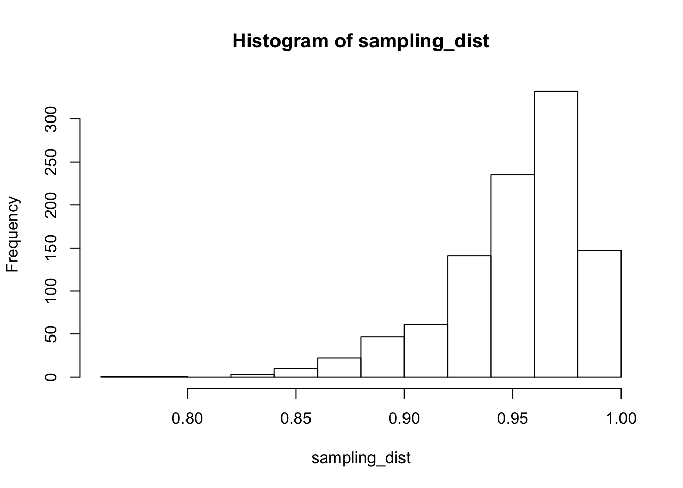
min(sampling_dist) #Smallest percentage of future values in prediction interval## [1] 0.7742589mean(sampling_dist) #Expected percentage of future values in prediction interval## [1] 0.9506352mean(sampling_dist < 0.9) #percentage of times that prediction interval predicts less than 90% of future values## [1] 0.084density(sampling_dist)$x[which.max(density(sampling_dist)$y)] #Most likely percentage of future values contained in prediction interval## [1] 0.9673389The histogram of attained probabilities that a prediction interval will contain future data explains what is going on. The probabilities have expected value of 0.95, but the distribution is skew. The most likely outcome seems to be that the prediction interval contain about 97% of future data, but there is about a 8% chance that it will contain less than 90% of future data. The minimum amount of future data contained (in this sample size of 1000) is 77%!
Sample Size
I have heard people say that the benefit of having more samples is that the prediction intervals get narrower. That is true, but also true is that a 95% prediction interval is also much more likely to contain about 95% of future values! Let’s see what happens when we have 300 and 3000 data points, rather than 30:
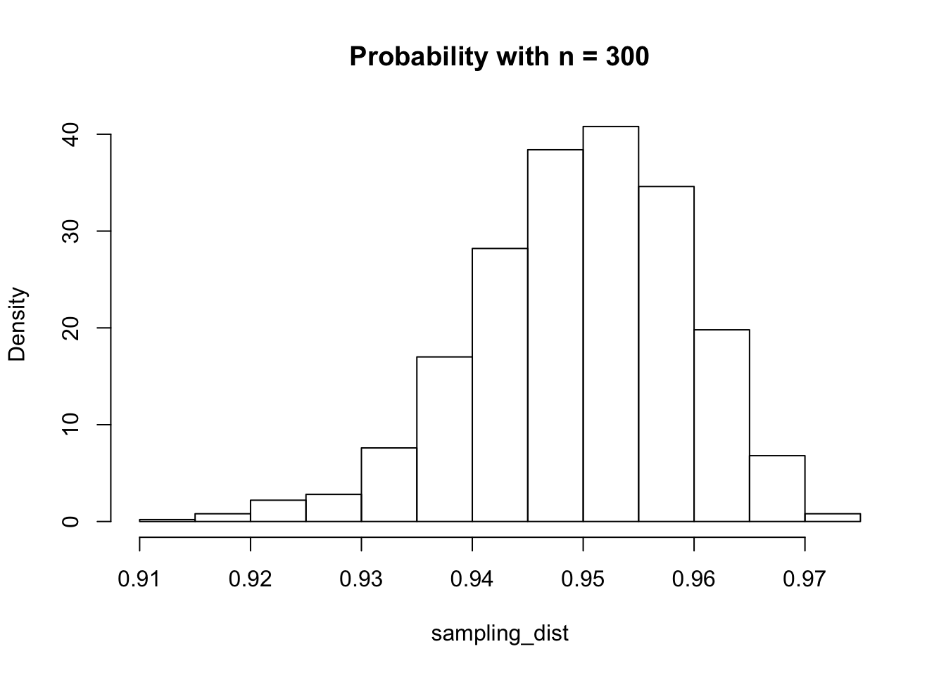
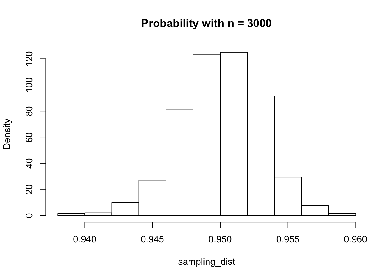
Table of Standard Deviations
Finally, we estimate the standard deviation of the sampling distribution of the probability that a future value will be in a prediction interval for various sample sizes.
sample_sizes <- c(10, 20, 50, 100, 200, 500, 1000, 2000, 5000)
sds <- sapply(sample_sizes, function(n) {
  sd(replicate(1000, {
    x <- runif(n, 0, 10)
    y <- 1 + 2 * x + rnorm(n, 0, 3)
    mod <- lm(y~x)
    pre <- predict(mod, newdata = data.frame(x = 5), interval = "pre")
    pnorm(pre[3], 11, 3) - pnorm(pre[2], 11, 3)
  }))
})
knitr::kable(data.frame(`Sample Size` = sample_sizes, `Standard Dev` = sds))| Sample.Size | Standard.Dev |
|---|---|
| 10 | 0.0705585 |
| 20 | 0.0386866 |
| 50 | 0.0242093 |
| 100 | 0.0162205 |
| 200 | 0.0117437 |
| 500 | 0.0071819 |
| 1000 | 0.0050827 |
| 2000 | 0.0037369 |
| 5000 | 0.0022930 |