Copula Sampling

One variable example

To start, let’s remind ourselves about the “universality of the uniform” for one-dimensional data. If \(X\) is a (continuous) random variable with distribution function \(F\), then \(F(X)\) is uniform(0, 1). Let’s illustrate this by sampling from an exponential rv with rate 1, applying \(F(x) = 1 - e^{-x}\) and plotting a histogram.

exp_sample <- rexp(10000)
transformed_data <- 1 - exp(-exp_sample)
hist(transformed_data)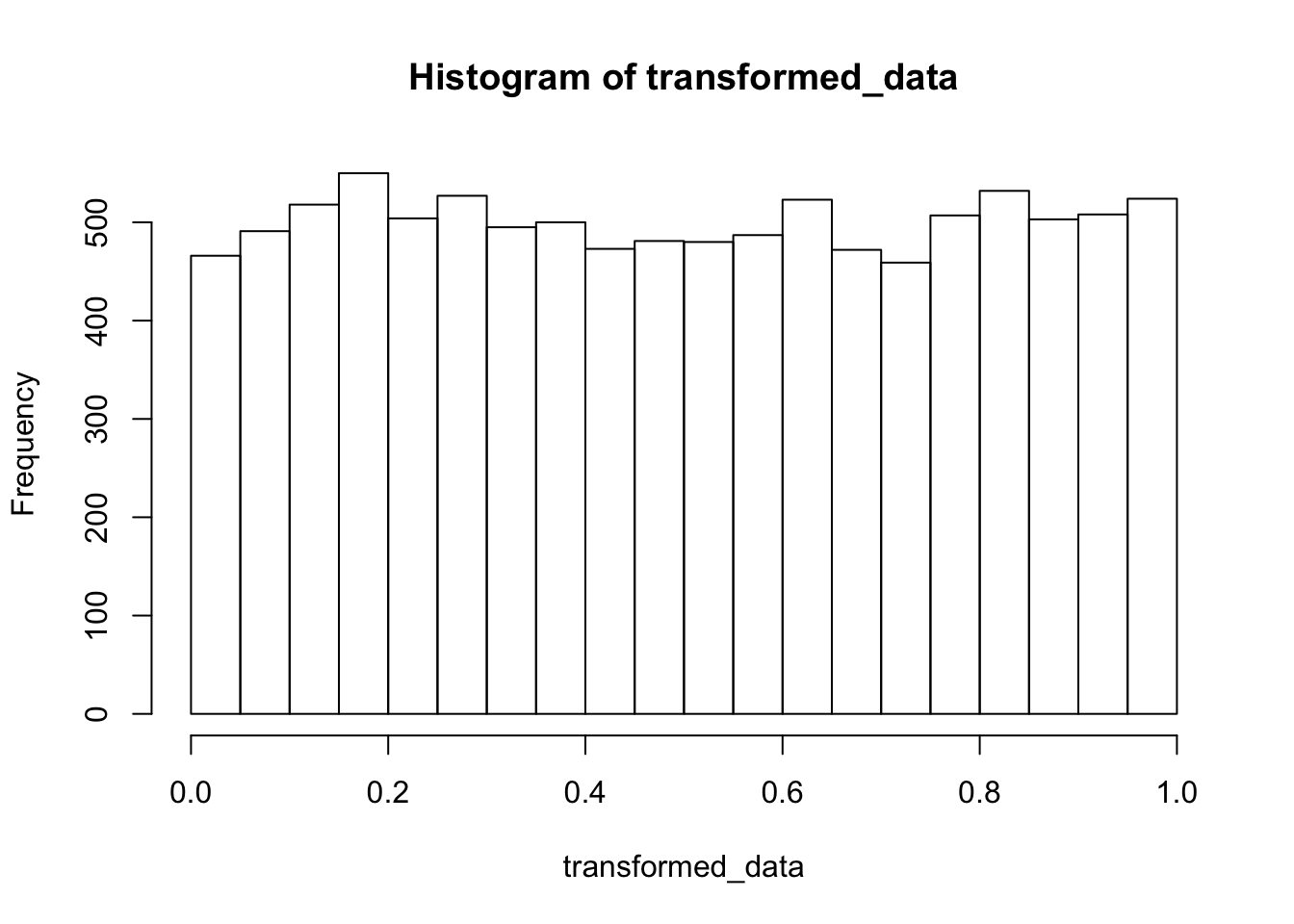

Looks convincingly uniform to me!

The flip side of this is that if we want to sample from an exponential rv, we can sample from a uniform(0,1) and apply \(F^{-1}\). Note that in this case, \(F^{-1}(x) = \log \frac{1}{y - 1}\).

uniform_sample <- runif(10000, 0, 1)
exp_sample <- log(1/(1 - uniform_sample))
hist(exp_sample, probability = TRUE)
curve(dexp(x), add = TRUE)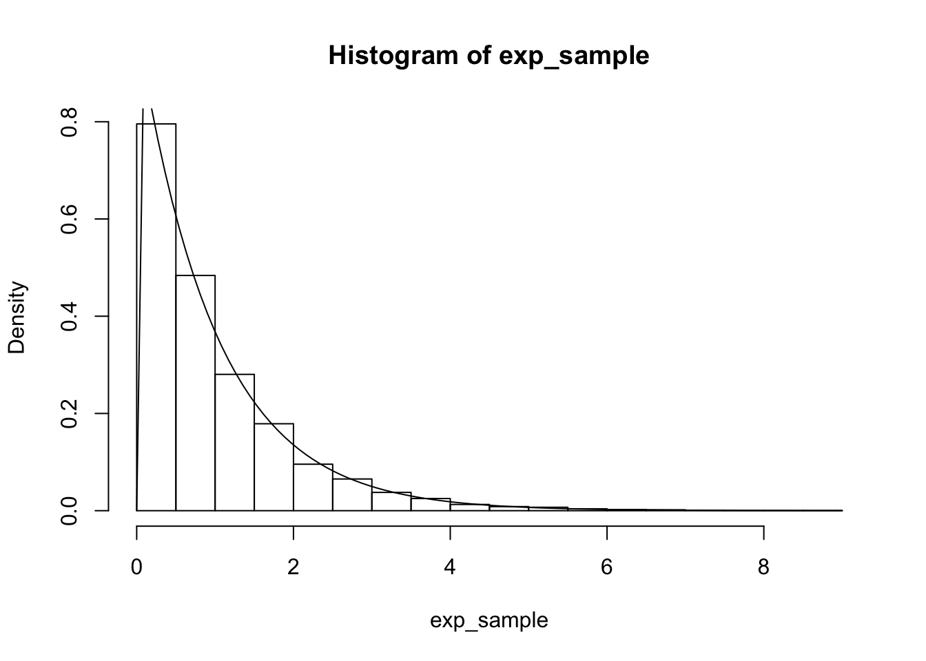

Convincing enough to me!

Multivariate Example

There is a higher dimensional version of the universality of the uniform, but it is trickier. Basically, if you start with \(X\) and \(Y\) with joint cdf \(F(x, y)\) and marginal distribution functions \(F_X\) and \(F_Y\), then \(F_X(X)\) and \(F_Y(Y)\) are both uniform(0, 1). If \(X\) and \(Y\) are independent, then we can proceed as before, but if they are dependent, then we need to encode that dependence. That’s where copulas come in.

We define the copula by \[ C(x, y) = P(F_X(X) \le x, F_Y(Y) \le y) \] Note that if \(X\) and \(Y\) are independent, then \(C(x,y) = xy\) since the probabilities just multiply (and remember \(F_X(X)\) is uniform(0, 1)!). However, in general, this will not be the case.

Let’s look at an example. We consider the joint density given by \[ f(x, y) = \begin{cases} 3x & 0\le y \le x \le 1 \\ 0&{\text{otherwise}} \end{cases} \] which has marginal distribution functions \[ F_X(x) = x^3 \] and \[ F_Y(y) = \frac 32 y - \frac 12 y^3 \] So, if we want to visualize a copula, we would need to sample from the original joint distribution: (I am using rejection sampling here)

sim_data <- matrix(c(0,0), ncol = 2)

for(i in 1:10000) {
  a <- runif(2)
  if(runif(1,0,3) < 3*a[1] && a[2] <= a[1])
    sim_data <- rbind(sim_data, a) 
}
sim_data <- sim_data[-1,]

Then, we sample from \((F_X(X), F_Y(Y))\) by just applying \(F_X\) and \(F_Y\) coordinatewise:

sd2 <- sim_data
sd2[,1] <- sd2[,1]^3
sd2[,2] <- 3/2 * sd2[,2] - 1/2 * sd2[,2]^3

You can check that the marginals are approximately uniform by doing histograms, but what we really want to do is to visualize the copula, so we do a scatterplot of the copula:

plot(sd2)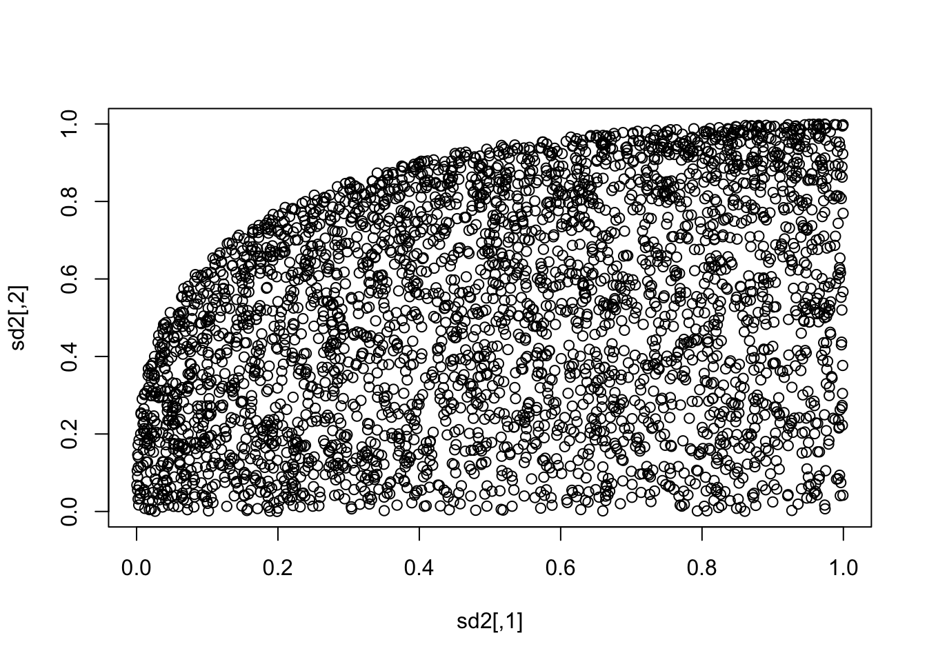

Or, we can do something fancier:

ggsd <- data.frame(sd2)
names(ggsd) <- c("x", "y")
library(ggplot2)
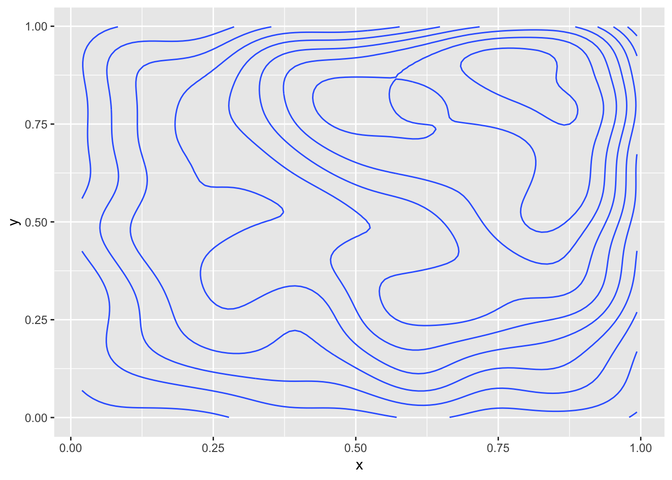
ggplot(ggsd, aes(x, y)) + 
  geom_density2d(bins = 9)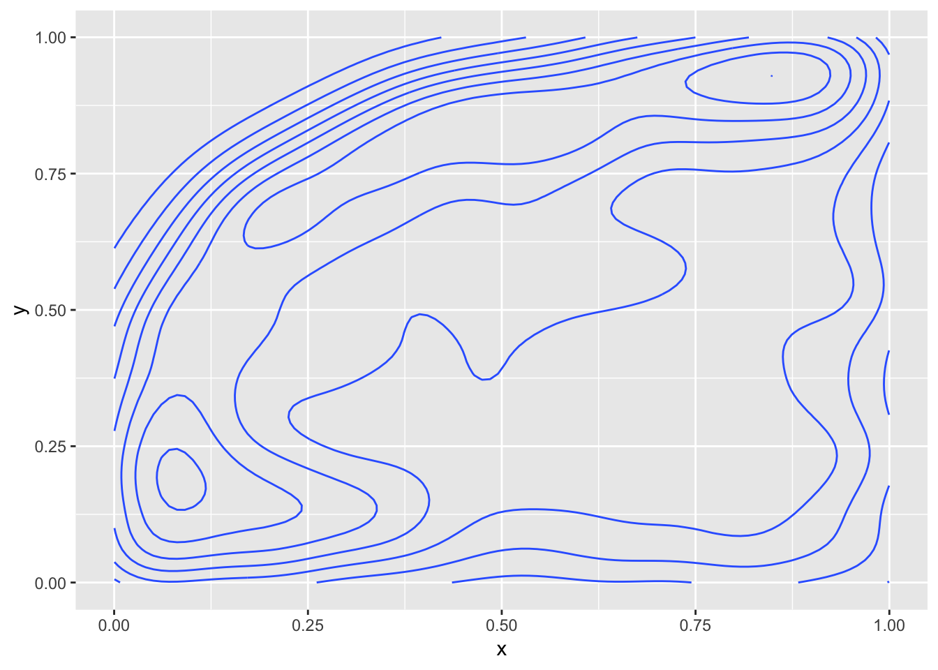

Doing the inverse!

OK, now that I know what the heck a copula is (sort of), and have at least seen one in the wild, let’s turn to what I was actually interested in. I had heard that you can sample from joint distributions by sampling from the copula and then applying the inverse of the distribution functions to each variable separately. Well, that doesn’t sound so bad. But, how do you sample from the copula?

Let’s look at an example. Suppose that \(X\) and \(Y\) have joint density function given by \[ f(x, y) = \begin{cases} x + y & 0\le x \le 1, 0 \le y \le 1\\0& {\text{otherwise}} \end{cases} \] So the joint cdf is \[ F(x, y) = \frac {1}{2} \bigl(x^2 y + x y^2\bigr) \] and the marginal distribution functions are given by. \[ F_X(x) = F_Y(x) = \frac 12 \bigl(x^2 + x\bigr) \]

Now, we could just figure out the inverse of the functions \(F_X\) and \(F_Y\), but I found this really cool answer here by Mike Axiak. Thanks! I am just stealing it almost 100%, even to the point of not changing the parameters beyond making them work in my situation…

inverse = function (f, lower = -100, upper = 100) {
  function (y) uniroot((function (x) f(x) - y), lower = lower, upper = upper)$root
}

FX_inverse <- inverse(function (x) x^2/2 + x/2, 0, 100) 
FY_inverse <- FX_inverse

I went ahead and defined \(F_Y\) inverse, even though it is the same in this case. Now, we define the joint density function and the copula:

cc <- function(x, y) 1/2 * (x^2 * y + x * y^2) #joint density function
cop <- function(u1, u2) cc(FX_inverse(u1), FY_inverse(u2)) #copula

Applying the answer I referenced above, we can sample from the copula in the following way. Note, it is very slow, but I am just looking for something that I understand at all.

library(numDeriv)
get_u1 <- function(u2, cop) {
  ff <- function(x) cop(x, u2)
  #library(numDeriv)
  xs <- seq(0.01, 0.99, length.out = 100)
  ys <- sapply(xs, function(z) {
    u2 <- z
    ff <- function(x) cop(x, u2)
    grad(ff, z)
  })
  u1 <- xs[which.max(ys  > runif(1))]
  u1
}

So, to get a single sample from the copula, we would use

u2 <- runif(1)
c(get_u1(u2, cop), u2)

## [1] 0.8811111 0.9386429

Now, let’s go get a Diet Coke from QuickTrip while we get 1000 samples from the copula.

sim_data <- matrix(c(0, 0), ncol = 2)
for(i in 1:1000) {
  u2 <- runif(1)
  sim_data <- rbind(sim_data, c(get_u1(u2, cop), u2))
}

Then, to get a sample from the original data, we would just apply the inverse distribution functions. For some reason, I couldn’t get these to vectorize, so I am using sapply.

sample_data <- sim_data[-1,]
sample_data[,1] <- sapply(sample_data[,1], function(x) FX_inverse(x))
sample_data[,2] <- sapply(sample_data[,2], function(x) FY_inverse(x))
plot(sample_data) #This is our sample from the distribution!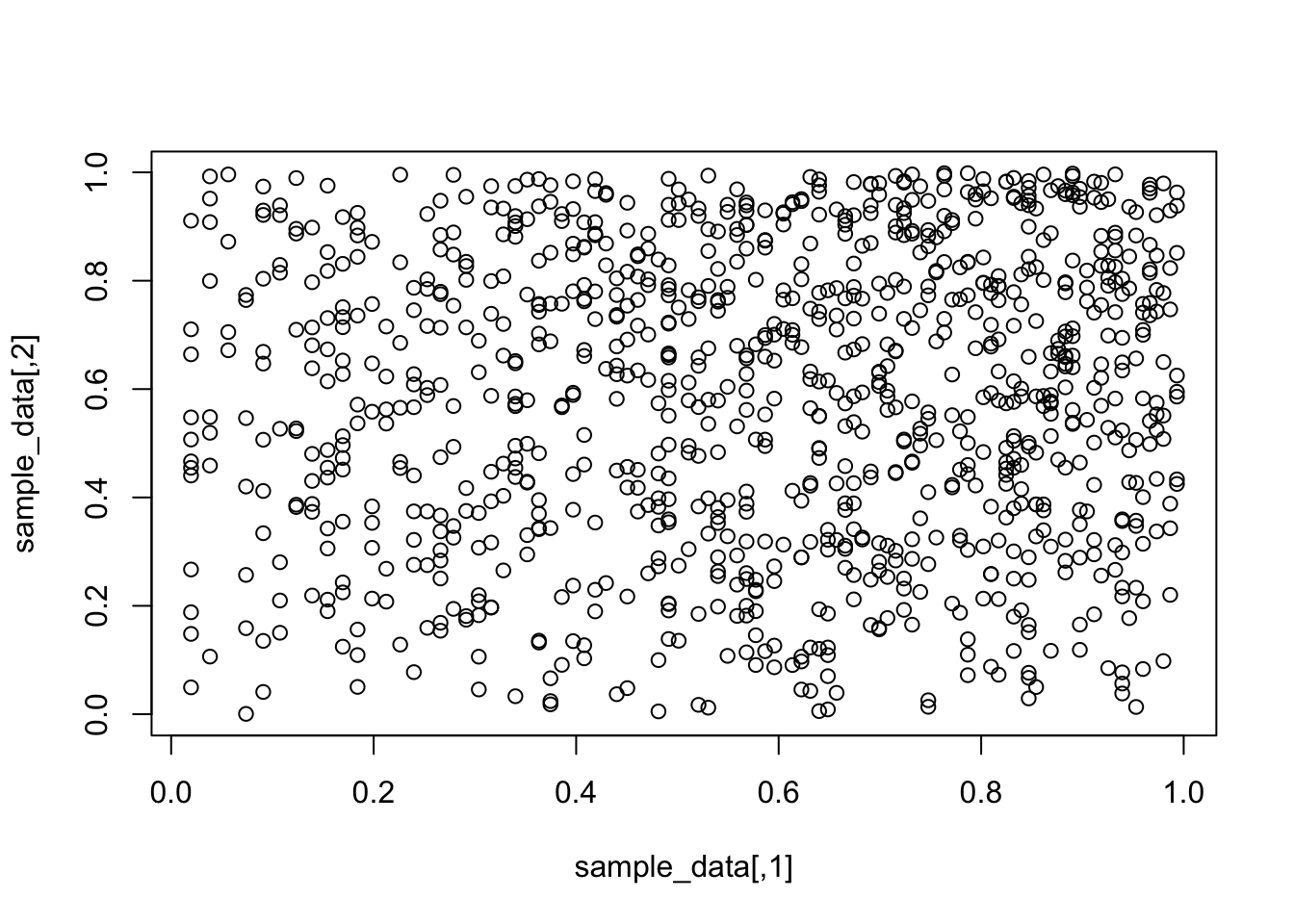

Another visualization:

ggsd <- data.frame(sample_data)
names(ggsd) <- c("x", "y")
ggplot(ggsd, aes(x, y)) + 
  geom_density2d(bins = 10)