On power and effect size

Introduction

I have seen a lot of tweets on my feed about power and effect size. I wanted to think about those things carefully, so I did some reading and am writing down some thoughts. An interesting paper that I read on this is here The takeaway is that studies that are underpowered, yet still obtain statistically significant results, will tend to overestimate the effect size.

Simulations

Let’s imagine that we are doing a hypothesis test of \(\mu = 0\) versus \(\mu \not = 0\), and our underlying population is normal with mean 1 and standard deviation 3. If we take a sample of size 30 and test at the \(\alpha = .05\) level, then our power is about 42%. We note that the true (Cohen’s \(d\)) effect size here is 1/3.

power.t.test(n = 30, delta = 1, sd = 3, sig.level = .05, type = "one")

## 
##      One-sample t test power calculation 
## 
##               n = 30
##           delta = 1
##              sd = 3
##       sig.level = 0.05
##           power = 0.4228091
##     alternative = two.sided

OK, now let’s run some simulations. This takes a sample of size 30 from normal with mean 1 and sd 3, and does a t-test. If it is significant at the \(\alpha = .05\) level, then the mean and sd are computed of the original data.

dat <- rnorm(30, 1, 3)
library(dplyr)
library(ggplot2)
sim_data <- do.call(rbind.data.frame, lapply(1:10000, function(x) {
  dat <- rnorm(30, 1, 3)
  if(t.test(dat)$p.value < .05) { 
       data.frame(mean = mean(dat), sd = sd(dat))
  } else {
       data.frame(mean = NA, sd = NA)
  }
})) %>% tidyr::drop_na()

Now, let’s see what the Cohen’s \(d\) values were, for the significant tests.

sim_data <- mutate(sim_data, cohensd = mean/sd)
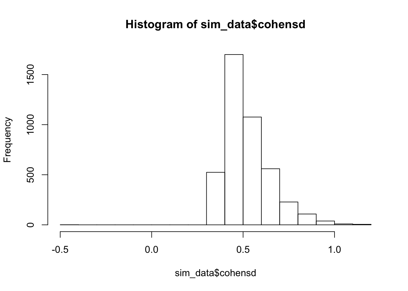
hist(sim_data$cohensd)

As we can see, the most likely outcome is just under 0.5, rather than the true value of 1/3. So, this is a biased way of computing Cohen’s \(d\).

The mean Cohen’s \(d\) is

mean(sim_data$cohensd)

## [1] 0.5224815

Now, let’s compare that to the case that the test has power of 0.8.

power.t.test(delta = 1, sd = 3, sig.level = .05, power = 0.8, type = "one")

## 
##      One-sample t test power calculation 
## 
##               n = 72.58407
##           delta = 1
##              sd = 3
##       sig.level = 0.05
##           power = 0.8
##     alternative = two.sided

sim_data <- do.call(rbind.data.frame, lapply(1:10000, function(x) {
  dat <- rnorm(73, 1, 3)
  if(t.test(dat)$p.value < .05) { 
       data.frame(mean = mean(dat), sd = sd(dat))
  } else {
       data.frame(mean = NA, sd = NA)
  }
})) %>% tidyr::drop_na()
sim_data <- mutate(sim_data, cohensd = mean/sd)
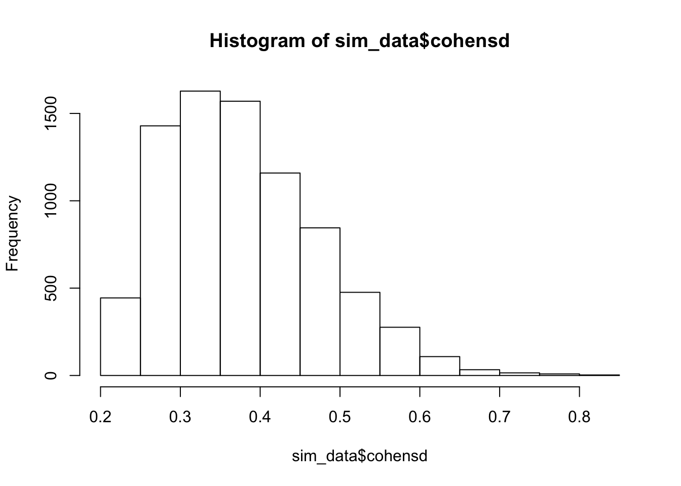
hist(sim_data$cohensd)

mean(sim_data$cohensd)

## [1] 0.3785638

Still biased, but now the most likely outcome is a value that is approximately correct.

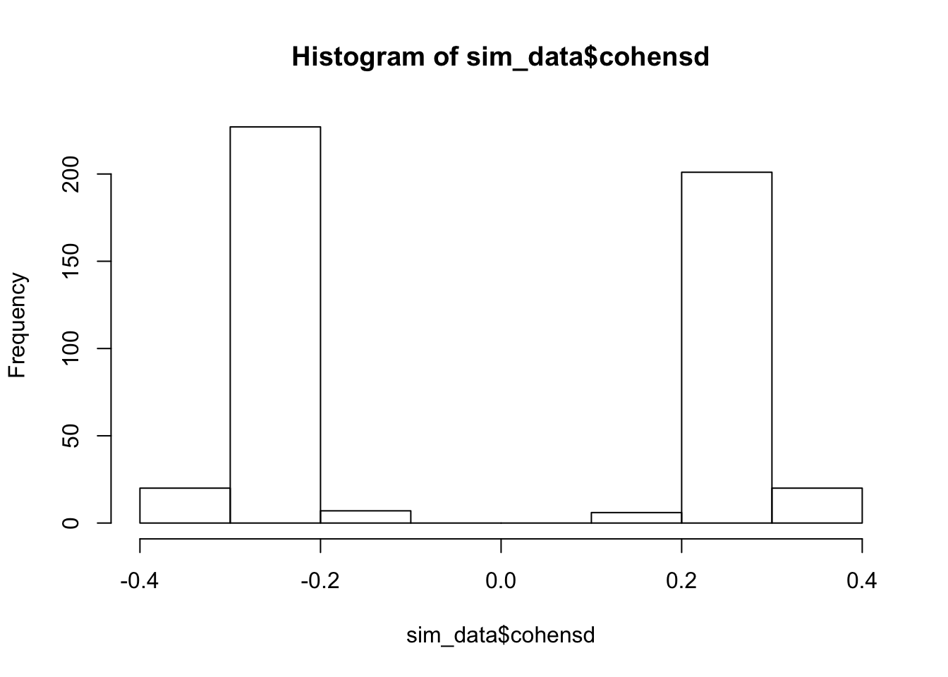
Finally, we show an example where the test is really underpowered; that is, \(H_0\) is actually true.

sim_data <- do.call(rbind.data.frame, lapply(1:10000, function(x) {
  dat <- rnorm(100, 0, 3)
  if(t.test(dat)$p.value < .05) { 
       data.frame(mean = mean(dat), sd = sd(dat))
  } else {
       data.frame(mean = NA, sd = NA)
  }
})) %>% tidyr::drop_na()
sim_data <- mutate(sim_data, cohensd = mean/sd)
hist(sim_data$cohensd)

mean(abs(sim_data$cohensd))

## [1] 0.2388848

Sample size

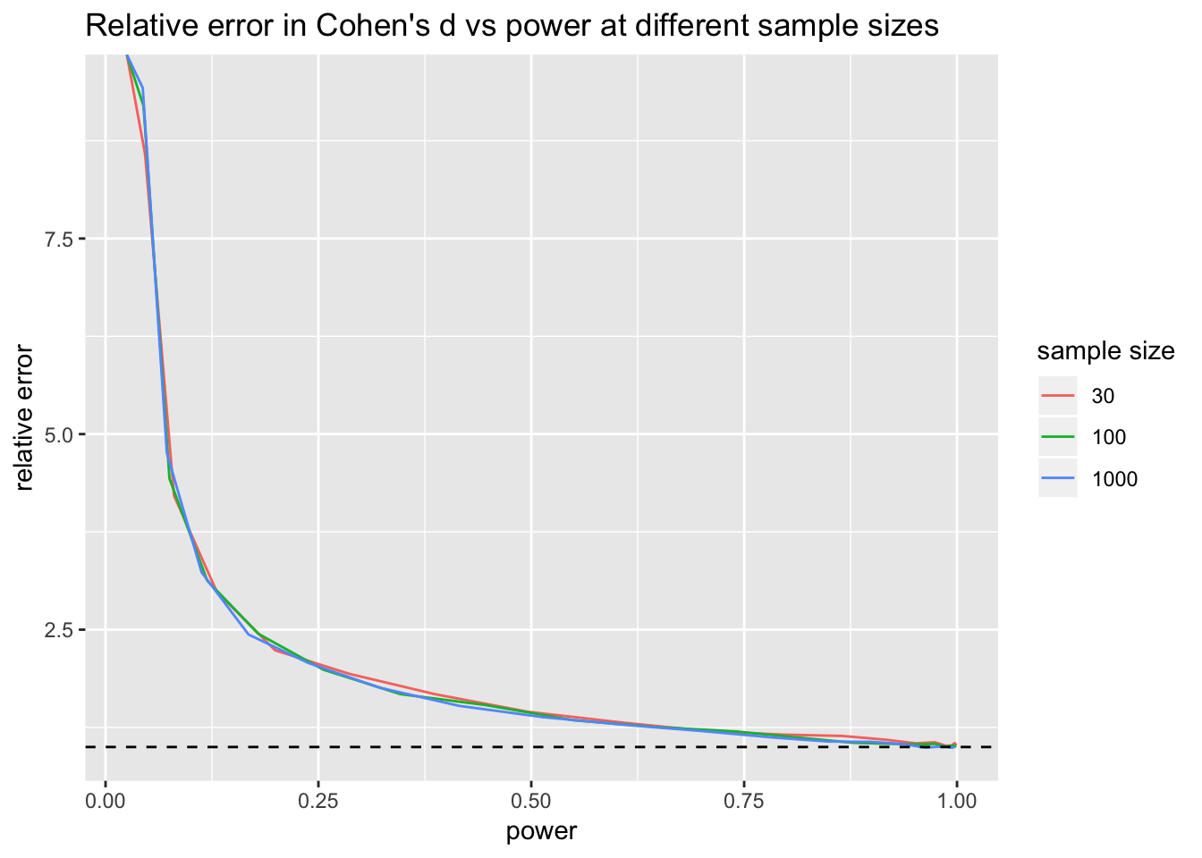
I haven’t done the math on how power and bias in estimation of effect size are related. I tought, though, that the sample size might also play a roll. So, I ran an analysis of relative error in effect size estimate for different sample sizes and different powers. Then, I plotted them below. You can see the (ugly) code I used to do this on my github account if you are so inclined. Bottom line, turns out I was wrong. The bias in the estimation of effect size seems to only depend on the power of the test.

The graph below plots estimated mean Cohen’s \(d\) at various powers for sample sizes of \(n = 30, 100\) and \(1000\). That is, the plot is of the estimated value of Cohen’s \(d\) divided by the true value. For my purposes, the estimated value was computed as the sample mean of the data divided by the sample standard deviation of the data, while the true value was the true mean of the underlying population divided by the true standard deviation of the underlying population. Recall that we are testing \(H_0: \mu = 0\) so the true mean is also the difference between the true mean and \(\mu_0\).